File:Butterworth response.png
Dettagli
| Descrizione |
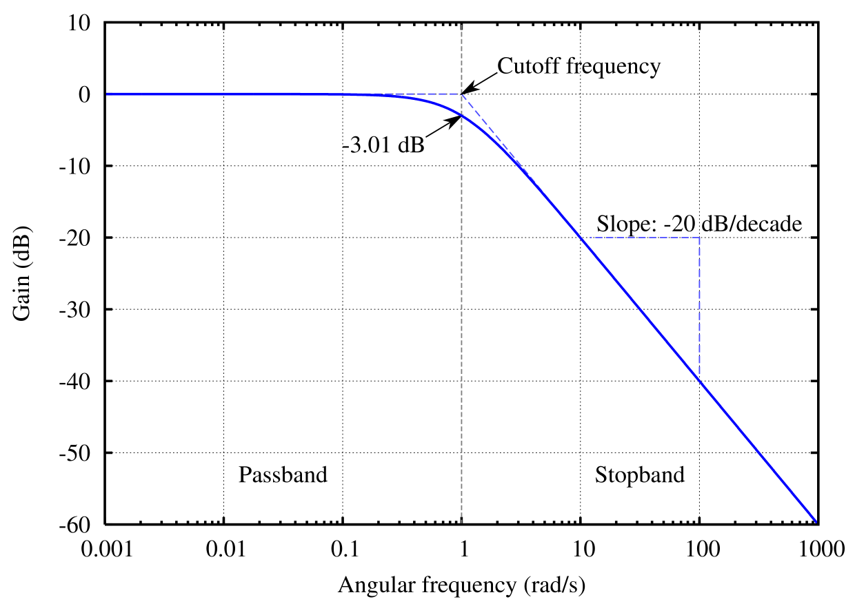
English: The frequency response of a Butterworth filter with logarithmic axes (Bode plot) and various labels. Cutoff frequency is normalized to 1 rad/s. Gain is normalized to 0 dB in the passband.
Many orders on one plot: File:Butterworth orders.png. Version with no text available at File:Butterworth plain.png, though you should probably just modify the source code and regenerate it in your own language. See Wikipedia graph-making tips. Generated in gnuplot with the script below (save as butterworth.plt and then open in gnuplot). Then I opened the butterworth.ps file in a text editor to edit the line colors and linestyles, as per this description. This avoids needing to open in proprietary software, and really isn't that difficult (especially if you don't know the commands in the proprietary software either). ;-) Identify the lines easily by their color (the arrow is currently magenta and I want it to be black. Ah, there is the entry with 1 0 1, red + blue = magenta) or by using the gnuplot linestyle−1. (For instance, gnuplot's linestyle 3 corresponds to the ps file's /LT2.) Then you can edit the colors and dashes by hand. I changed the original: /LT0 { PL [] 1 0 0 DL } def
/LT1 { PL [4 dl 2 dl] 0 1 0 DL } def
/LT2 { PL [2 dl 3 dl] 0 0 1 DL } def
/LT3 { PL [1 dl 1.5 dl] 1 0 1 DL } def
into this: /LT0 { PL [] 0 0 1 DL } def
/LT1 { PL [4 dl 2 dl] 0.5 0.5 0.5 DL } def
/LT2 { PL [6 dl 3 dl] 0.3 0.3 1 DL } def
/LT3 { PL [] 0 0 0 DL } def
/LT4–/LT8 I left unchanged. (I don't know what they're used for anyway.) /LTw, /LTb, and /LTa are for the grid lines and such.To convert the PostScript file to PNG:
|
| Data | 26 giugno 2005 (data di caricamento) |
| Fonte | Opera propria |
| Autore | Omegatron |
| Altre versioni |
|
| gnuplot source | click to expand
set samples 2001
set terminal postscript enhanced landscape color lw 2 "Times-Roman" 20
set output "butterworth.ps"

# Butterworth amplitude response and decibel calculation.  n is the order, which is just 1 in this image.
G(w,n) = 1 / (sqrt(1 + w**(2*n)))
dB(x) = 20 * log10(abs(x))

# Gridlines
set grid

# Set x axis to logarithmic scale
set logscale x 10

# Set range of x and y axes
set xrange [0.001:1000]
set yrange [-60:10]

# Create x-axis tic marks once per decade (every multiple of 10)
set xtics 10

# Use 10 x-axis minor divisions per major division
set mxtics 10

# Axis labels
set xlabel "Angular frequency (rad/s)"
set ylabel "Gain (dB)"

# No need for a key
set nokey #0.1,-25

# Frequency response's line plotting style
set style line 1 lt 1 lw 2

# Draw a separator between passband and stopband and label them
set style line 2 lt 2 lw 1
set style arrow 2 nohead ls 2
set arrow 3 from 1,-60 to 1,10 as 2

# Label coordinates are relative to the graph window, not to the function, centered at the 1/4 and 3/4 width points
set label 1 "Passband" at graph 0.25, graph 0.1 c
set label 2 "Stopband" at graph 0.75, graph 0.1 c

# Asymptote lines and slope lines are the same "arrow" style
set style line 3 lt 3 lw 1
set style arrow 3 nohead ls 3

# Draw asymptote lines
set arrow 1 from 1,0 to 1000,-60 as 3
set arrow 2 from .001,0 to 1,0 as 3

# -3 dB arrow style and arrow
set style line 4 lt 4 lw 1
set style arrow 4 head filled size screen 0.02,15,45 ls 4
set arrow 4 from 2,3 to 1,0 as 4

# "Cutoff frequency" label uses same coordinates as the function
set label 3 "Cutoff frequency" at 2,4 l

# "-3 dB" label
set arrow 5 from 0.5,-6 to 1,-3 as 4
set label 4 "-3.01 dB" at 0.5,-7 r

# Draw slope lines and label
set arrow 6 from 100,-20 to 12,-20 as 3
set arrow 7 from 100,-20 to 100,-39 as 3
set label 5 "Slope: -20 dB/decade" at 100,-18 c

# Plot the filter response
plot \
     dB(G(x,1)) ls 1  title "1st-order response"
|


|
File:Butterworth response.svg è una versione vettoriale di questo file. Dovrebbe essere usata quella versione al posto di questo file PNG, quando sia migliore.
File:Butterworth response.png → File:Butterworth response.svg
Per maggiori informazioni, vedi Help:SVG. |
 |
Licenza
- Tu sei libero:
- di condividere – di copiare, distribuire e trasmettere quest'opera
- di modificare – di adattare l'opera
- Alle seguenti condizioni:
- attribuzione – Devi fornire i crediti appropriati, un collegamento alla licenza e indicare se sono state apportate modifiche. Puoi farlo in qualsiasi modo ragionevole, ma non in alcun modo che suggerisca che il licenziante approvi te o il tuo uso.
- condividi allo stesso modo – Se remixi, trasformi o sviluppi il materiale, devi distribuire i tuoi contributi in base alla stessa licenza o compatibile all'originale.

|
È permesso copiare, distribuire e/o modificare questo documento in base ai termini della GNU Free Documentation License, Versione 1.2 o successive pubblicata dalla Free Software Foundation; senza alcuna sezione non modificabile, senza testo di copertina e senza testo di quarta di copertina. Una copia della licenza è inclusa nella sezione intitolata Testo della GNU Free Documentation License. |
Cronologia del file
Fare clic su un gruppo data/ora per vedere il file come si presentava nel momento indicato.
| Data/Ora | Miniatura | Dimensioni | Utente | Commento | |
|---|---|---|---|---|---|
| attuale | 18:45, 23 lug 2005 | | 1 240 × 880 (86 KB) | wikimediacommons>Omegatron | split the cutoff frequency markers |
Utilizzo del file
Le seguenti 2 pagine usano questo file: